SciPy Multidimensional image processing

Image computation and analysis are commonly thought of as activities on 2-D arrays of values. However, there are a few fields where higher-dimensional images must be evaluated. Medical imaging and molecular imaging are good examples of these. Because of its intrinsic multi-dimensional nature, numpy is highly suited for this sort of application. The scipy.ndimage package contains a number of image manipulation and analysis routines that work with arrays of any size. Methods for linear filtering and non-linear filtering, B-Spline interpolation, object measurements, and binary morphology are currently included in the packages.

Functions of SciPy Multidimensional Image Processing Sub-Package

Some attributes are shared by all functions. Notably, with the output option, all functions allow for the specification of a returned array. This input allows you to define an array which will be updated in-place with the operation's outcome. The output is not provided in this scenario. Using the result argument is generally more efficient because the output is stored in an existing array.

The kind of arrays generated is determined by the operation; however it is usually the same as the type of input. The type of the output is equivalent to the form of the specified output parameter if the output is utilized. It is still feasible to describe what the output result should be if no output parameter is specified. Simply assign the required numpy data type to the output parameter to accomplish this.

Filters

The functions in this section all apply spatial filtering to the provided array: the elements in the output are a function of the values in the corresponding input element's neighborhood. The filter kernel is the name given to this group of elements, which is usually rectangular in shape, however can have any shape. By giving a filter through the footprint argument to several of the functions listed below, you can define the kernel's footprint.

convolve(input, weights[, output, mode, ...])	Multiple-dimensional convolution.
convolve1d(input, weights[, axis, output, ...])	This function computes a convolution in 1-D along the supplied axis.
correlate(input, weights[, output, mode, ...])	On numerous levels, there is a correlation.
gaussian_filter(input, sigma[, order, ...])	Gaussian filter in several dimensions.
gaussian_filter1d(input, sigma[, axis, ...])	Filter with a one-dimensional Gaussian distribution.
gaussian_gradient_magnitude(input, sigma[, ...])	Gaussian derivatives are used to calculate the magnitude of multidimensional gradients.
generic_gradient_magnitude(input, derivative)	Using a gradient function provided, calculate the magnitude of the gradient.
generic_laplace(input, derivative2[, ...])	Using a second derivative function provided, create an N-D Laplace filter.
laplace(input[, output, mode, cval])	Based on approximate second derivatives, N-D Laplace filter.

Fourier filters

Filtering actions within Fourier domain are performed by the functions given in this section. As a result, the initial array of such a method should be consistent with an inverse Fourier transform function, like the numpy.fft module's functions. As a result, we must work with arrays that are the result of either a real or a complex Fourier transform.

fourier_ellipsoid(input, size[, n, axis, output])	A multidimensional ellipsoid is used by this function for Fourier filtering.
fourier_gaussian(input, sigma[, n, axis, output])	Multiple-dimensional Fourier filter Gaussian.
fourier_shift(input, shift[, n, axis, output])	This function is used for N-dimensional Fourier shift filtering.

Interpolation

The many interpolation functions based on B-spline theory are described in this section.

affine_transform(input, matrix[, offset, ...])	It's best to employ an affine transformation.
geometric_transform(input, mapping[, ...])	You can use whatever geometric transformation you want.
map_coordinates(input, coordinates[, ...])	This function will map the array you will input to new coordinates using interpolation.
rotate(input, angle[, axes, reshape, ...])	An array will be rotated.
shift(input, shift[, output, order, mode, ...])	An array's order will be changed.
spline_filter1d(input[, order, axis, ...])	This function will compute a1-D spline filter along the axis of your choice.
zoom(input, zoom[, output, order, mode, ...])	Zooming in and out of an array is done.

Measurements

The attributes of individual items can be measured provided an array of labeled objects. The find objects method can be used to build a list of slices that provide the tiniest sub-array that completely covers each item for each object. The index parameter is supported by all of the measurement functions mentioned below to specify which object(s) should be evaluated. The default index value is None. This means that all elements with a label greater than 0 should be handled as a single item and measured as a whole. As a result, the labels array is interpreted as a mask specified by the elements larger than zero in this example.

center_of_mass(input[, labels, index])	This function will compute the centre of mass of an array's values at the labels.
extrema(input[, labels, index])	This function will compute the minimums and maximums of an array's values at each label, as well as their positions.
find_objects(input[, max_label])	In a tagged array, find objects.
histogram(input, min, max, bins[, labels, index])	This function will provide the histogram of an array's values, at labels (optionally).
label(input[, structure, output])	In an array, label the features.
maximum(input[, labels, index])	This function will compute the maximum of an array's values across labelled regions.
maximum_position(input[, labels, index])	This function will return the maximum values' positions from all array values at their labels.
labeled_comprehension(input, labels, index, ...)	For i in index, almost equal to [func(input[labels == I

Morphology

Morphological processing of image is a set of non-linear processes that deal with the structure or morphology of picture features.

binary_closing(input[, structure, ...])	With the specified structuring element, multidimensional binary closing is performed.
binary_dilation(input[, structure, ...])	With the specified structuring element, multidimensional binary dilation is performed.
binary_erosion(input[, structure, ...])	With a particular structuring element, multidimensional binary erosion is possible.
binary_fill_holes(input[, structure, ...])	This function fills binary object's holes.
binary_hit_or_miss(input[, structure1, ...])	Hit-or-miss multidimensional binary transform.
binary_opening(input[, structure, ...])	With the specified structuring element, a N-D binary opening is created.
binary_propagation(input[, structure, mask, ...])	With the specified structural element, N-D binary propagation is performed.
black_tophat(input[, size, footprint, ...])	This function performs N-D black tophat filtering.

Some useful methods

Now we will discuss some useful functions.

scipy.ndimage.convolve

It performs multidimensional convolution. With the provided kernel, the array provided is convolved.

Parameters

1. input (array_like):- The array to be convolved.
2. weights (array_like):- Weights' array with equal dimensions as the input
3. output (array or dtype, optional):- The dtype of the array returned, or the array into which the result should be placed. An array having same dtype as supplied array is produced by default.
4. mode ({‘reflect’, ‘nearest’, ‘wrap’, ‘constant’, ‘mirror’}, optional):- The mode argument controls how the given array is stretched outside its bounds. The default mode is 'reflect.'
5. cval (scalar, optional):- If the mode is 'constant,' the value used to fill in the gaps between the input's edges. The default value is 0.0.
6. origin (int, optional):- Handles the origin of the original signal, that's where the first item of the output is produced by the filter. Negative values push the filter to the left, whereas positive values shift it to the right. The default value is 0.

scipy.ndimage.gaussian_filter

Gaussian filter in several dimensions.

Parameters

1. input (array_like):- The array to be filtered.
2. sigma (scalar or sequence of scalars):- The level of blurring is controlled by the standard deviation provided to the Gaussian function.
3. order (int or sequence of ints, optional):- The filter's order along every axis is specified as an integer sequence or as an unique value. Convolution using a Gaussian kernel corresponds to an order of 0. A positive order refers to convolution with a Gaussian's derivative.
4. output (array or dtype, optional):- The dtype of the array returned, or the array into which the result should be placed. An array having same dtype as supplied array is produced by default.
5. mode (str or sequence, optional):- When the filter spans a boundary, the mode parameter controls how the initial array is stretched. Multiple types can be defined along every axis by passing a series of modes with a size equal to the dimensions of the given array. 'reflect' is the default value.
6. cval (scalar, optional):- If the mode is 'constant,' the value used to fill in the gaps between the input's edges. The default value is 0.0.
7. truncate (float):- At this many standard deviations, truncate the filter. The default value is 4.0.

scipy.ndimage.fourier_ellipsoid

N-D ellipsoid Fourier filter. The fourier transforms of an ellipsoid of provided sizes is multiplied by the array.

Parameters

1. input (array_like):- The array to be filtered.
2. size (float or sequence):- The dimension of the filtering box. The size of a float is equal for all axes. If you're using a sequence, size must have 1 value for every axis.
3. n (int, optional):- The input is considered to be the output of a complex fft if n is a negative number (the default). The input is presumed to be the outcome of a real fft if n is greater or equal to zero. The size of the array preceding transformation in the real transform direction is represented by n.
4. axis (int, optional):- The axis on which the real transform is performed.
5. output (ndarray, optional):- If this option is selected, the output of filtering the input is stored in this array. In this situation, none is returned.

scipy.ndimage.zoom

An array can be zoomed using this function. The array is scaled using the spline interpolation of the desired order.

Parameters

1. input (array_like):- The array to be zoomed.
2. zoom (float or sequence):- Along the axes, specifies the zoom factor. When using a float, the zoom for each axis is the same. If you're using a series, zoom should only have one value per axis.
3. output (array or dtype, optional):- The dtype of the array returned, or the array into which the output should be placed. An array of the identical dtype as source is produced by default.
4. order (int, optional):- The default for spline interpolation order is 3. The order must be between 0 and 5.
5. mode ({‘grid-wrap’ , ‘reflect’, ‘constant’, ‘grid-constant’, ‘grid-mirror’, ‘nearest’, ‘mirror’, ‘wrap’}, optional):- The mode argument controls how the given array is stretched outside its bounds. The default value is 'constant.'
6. cval (scalar, optional):- If the mode is 'constant,' the value used to fill in the gaps between the input's edges. The default value is 0.0.
7. prefilter (bool, optional):- If a spline filter was employed to prefilter the given array before interpolation, this value is true. True is the default value. If order > 1, the output will be significantly blurred if this is set to False, except if the input is prefiltered.
8. grid_mode (bool, optional):- The distance between the pixel centres is zoomed if False. Otherwise, the full pixel extent is being used to calculate the distance.

scipy.ndimage.gaussian_laplace

Gaussian second derivatives are used for this multidimensional Laplace filter.

Parameters

1. input (array_like):- The input array.
2. sigma (scalar or sequence of scalars):- The standard deviations  are supplied for Gaussian filter as a sequence for each axis, or as a single number for all axes, in which case they are identical.
3. output (array or dtype, optional):- The dtype of the array returned, or the array into which the output should be placed. An array of the identical dtype as source array is produced by default.
4. mode (str or sequence, optional):- When the filter spans a boundary, the mode parameter controls how the initial array is stretched. Different modes can be provided along every axis by passing a series of modes with a size equal to the number of dimensions of the given array. 'reflect' is the default value.
5. cval (scalar, optional):- If the mode is 'constant,' the value used to fill in the gaps between the input's edges. The default value is 0.0.

scipy.ndimage.uniform_filter

It filters multidimensional image uniformly

Parameters

1. input (array_like):- The array to be filtered.
2. size (int or sequence, optional):- The uniform filter's sizes are specified as a series for every axis or as a single value, in which situation the size is the same for all axes.
3. output (array or dtype, optional):- The dtype of the array returned, or the array into which the output should be placed. An array of the identical dtype as source array is produced by default.
4. mode (str or sequence, optional):- When the filter spans a boundary, the mode parameter controls how the initial array is stretched. Different modes can be provided along every axis by passing a series of modes with a size equal to the number of dimensions of the given array. 'reflect' is the default value.
5. cval (scalar, optional):- If the mode is 'constant,' the value used to fill in the gaps between the input's edges. The default value is 0.0.
6. origin (int or sequence, optional):- Controls where the filter is applied to the pixels of the input array. Positive values push the filter to the left, while negative values shift it to the right. Default value of this parameter centres the filter over the pixel, and the value is 0. Different shifts along each axis can be provided by passing a series of origins with a length equivalent to the total of dimensions of the given array.

Examples of Image Processing

Let us see the examples of the functions discussed in detail above.

Example – 1

Convolution is the technique of altering an image by implementing a kernel to every pixel and its local surroundings over the entire image in image processing. The kernel is a value matrix whose size and values affect the convolution process' transformation impact.

Input

import numpy as np
a = np.array([[5, 1, 8, 0],
              [9, 2, 10, 5],
              [3, 5, 7, 9],
              [8, 9, 4, 1]])
k = np.array([[2,2,2],[2,2,0],[2,0,0]])
from scipy import ndimage
c = ndimage.convolve(a, k, mode='constant', cval=0.0)
print(c)

Output

[[34 60 50 30]
 [40 70 72 42]
 [54 86 70 28]
 [44 40 28  2]]

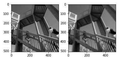
Example – 2

The fourier transform of an ellipsoid of given sizes is multiplied by the array.

Input

import scipy
import numpy
import matplotlib.pyplot as plt
fig, (axis1, axis2) = plt.subplots(1, 2)
image = scipy.misc.ascent()
plt.gray()  # this will show the image after filtering in grayscale
i = numpy.fft.fft2(ascent)
result = scipy.ndimage.fourier_ellipsoid(i, size=10)
result = numpy.fft.ifft2(result)
axis1.imshow(image)
axis2.imshow(result.real)  # the imaginary part is an artifact
plt.show()

Output

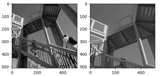
Example – 3

The image is zoomed using the requested order's spline interpolation. Spline interpolation is a sort of interpolation in which the interpolant is a spline, which is a special class of piecewise polynomial. Instead of fitting a singular, higher-degree polynomial to all the elements in one go, spline interpolation fits small subsets of the data using low-degree polynomials.

import scipy.misc
import scipy.ndimage
import matplotlib.pyplot as plt
fig = plt.figure()
plt.gray()
axis1 = fig.add_subplot(121)  # left hand side of figure
axis2 = fig.add_subplot(122)  # right hand side of figure
image = scipy.misc.ascent()
zoomed = scipy.ndimage.zoom(image, 1.5, mode='reflect')
axis1.imshow(image)
axis2.imshow(zoomed[0:512, 0:512])
print('Shape of original image: ', image.shape)
print('Shape of zoomed image: ', zoomed.shape)
plt.show()

Output

Shape of original image:  (512, 512)
Shape of zoomed image:  (768, 768)

Example – 4

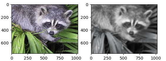
A Gaussian Filter is indeed a low-pass filter for reducing noise (noise are all components of high-frequency) and blurring image regions. The filter is designed as an Odd sized Symmetric Kernel which is processed through every pixel of the area of concern to generate the required effect.

Input

import scipy.ndimage
import scipy
import matplotlib.pyplot as plt
fig = plt.figure()
axis1 = fig.add_subplot(121)  # left hand side of figure
axis2 = fig.add_subplot(122)  # right hand side of figure
face = misc.face()
filtered = scipy.ndimage.gaussian_filter(ascent, sigma=8)
axis1.imshow(face)
axis2.imshow(filtered)
plt.show()

Output

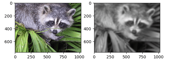
Example – 5

Uniform filtering works by replacing each pixel of the image with the average ('mean') value of its neighbours, including itself. As a result, pixel values that aren't typical of their surroundings are removed. Mean filtering is often mistaken for a convolution filter.

Input

import scipy.ndimage
import scipy.misc
import matplotlib.pyplot as plt
fig = plt.figure()
plt.gray()  # this will show the image after filtering in grayscale
axis1 = fig.add_subplot(121)  # left hand side of the figure
axis2 = fig.add_subplot(122)  # right hand size of the figure
image = scipy.misc.face()
filtered = scipy.ndimage.uniform_filter(image, size=20)
axis1.imshow(image)
axis2.imshow(filtered)
plt.show()

Output