SciPy Interpolation
The technique of determining a number between two endpoints on a line or a curve is known as interpolation. To recall what it implies, consider the initial part of the term, 'inter,' to imply 'enter,' which instructs us to examine 'within' the data we started with. Interpolation is a tool that is important not only in statistics, but also in science, business, and for predicting values that fall between two existent data points.

Investors and market analysts typically use interpolated data points to build a line chart. These charts, which are a key aspect of technical analysis, enable them visualize fluctuations in the cost of securities. While computer techniques are now widely used to produce these data points, interpolation is not really a new notion. Ancient astronomers in Mesopotamia and Asia Minor employed interpolation to bridge the gaps in their observations of the motions of the planets.
Interpolation may appear to be a complicated mathematical exercise, yet it is similar to machine learning in many respects.
- Begin with a small number of data points that relate to many factors.
- Use interpolation (so basically, make a model)
- Create a new function that can forecast any forthcoming or new point based on the interpolation.
So, the plan is to ingest, extrapolate, and forecast.
Let's say we have a finite number of observations for a two variables (a,b) with an uncertain (and nonlinear) connection, such as b = f. (a). We want to build a prediction function from this restricted data that can create value of y for any provided value of x (in the very same range which was used before for the interpolation).
Interpolation and Its Types
Interpolation is a method of creating data points from a set of data points. In Python SciPy, the scipy.interpolate module contains methods, univariate and multivariate and spline functions interpolation classes. Interpolation can be done in a variety of methods, including:
- 1-D Interpolation
- Spline Interpolation
- Univariate Spline Interpolation
- Interpolation with RBF
- Multivariate Interpolation
Interpolation in SciPy
1-D Interpolation
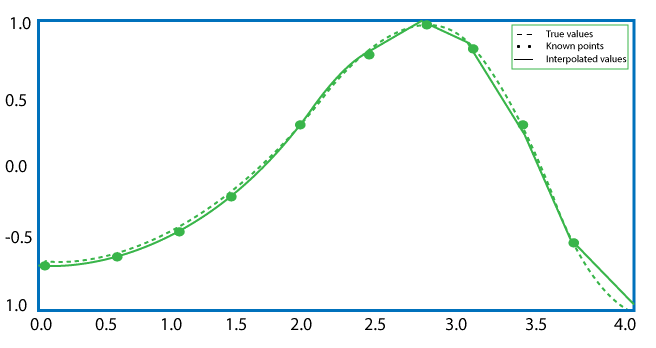
In contrast to univariate regression analysis, which finds the curve that provides a perfect fit to a sequence of two-dimensional data points, univariate interpolation identifies the curve that provides an exact match to a sequence of two-dimensional data sets. The data points are expected to be chosen from a one-variable function, hence it's termed univariate. Any form of function can be used as long as it delivers an accurate fit to the provided data points. Our decision should be founded on some previous knowledge of the events that lead to the formation of that set of points.
Univariate Interpolation SciPy Functions
| interp1d(x, y[, kind, axis, copy, …]) | Interpolate a one-dimensional function. |
| BarycentricInterpolator(xi[, yi, axis]) | For a set of points, the interpolating polynomial |
| KroghInterpolator(xi, yi[, axis]) | Polynomial interpolation for a series of points. |
| barycentric_interpolate(xi, yi, x[, axis]) | Polynomial interpolation convenience function. |
| krogh_interpolate(xi, yi, x[, der, axis]) | Polynomial interpolation convenience function. |
| CubicHermiteSpline(x, y, dydx[, axis, …]) | Values and first derivatives are matched using a piecewise-cubic interpolator. |
| PchipInterpolator(x, y[, axis, extrapolate]) | monotonic cubic interpolation PCHIP 1-D. |
| Akima1DInterpolator(x, y[, axis]) | Interpolator Akima |
| CubicSpline(x, y[, axis, bc_type, extrapolate]) | This function interpolates data using Cubic Spline |
| PPoly(c, x[, extrapolate, axis]) | In view of coefficients and breakpoints, a piecewise polynomial |
Piecewise linear, piecewise constant, polynomial, and spline are all examples of univariate interpolation. The same y-values are assigned to surrounding x-values in piecewise constant interpolation. Lines connect successive points in piecewise linear interpolation. spline interpolation or Polynomial interpolation can be used to make it smoother.
Multivariate Interpolation
Multivariate interpolation involves interpolation on functions with more than one variable in numerical analysis; it is also termed as internal interpolation when the variates are space coordinates. In contrast to univariate interpolation, which fits two-dimensional data points, multivariate interpolation determines the surface that provides an accurate fit to a set of multidimensional data points. The data points are expected to be generated from a proper function of numerous variables, hence it's termed multivariate. In geostatistics, multivariate interpolation is used to construct a computerized elevation model from a series of points on the Earth's crust (for an instance depths in a hydrographic survey).
If available data is unstructured
| griddata(points, values, xi[, method, …]) | This function interpolates unstructured D-D data. |
| LinearNDInterpolator(points, values[, …]) | Unstructured D-D data is interpolated. |
| NearestNDInterpolator(x, y[, rescale, …]) | In N > 1 dimensions, piecewise linear interpolant. |
| CloughTocher2DInterpolator(points, values[, …]) | NearestNDInterpolator is a function that calculates the distance between two points (x, y). |
| RBFInterpolator(y, d[, neighbors, …]) | Interpolation using the radial basis function (RBF) over N dimensions. |
| Rbf(*args) | Interpolation using the radial basis function (RBF) over N dimensions. |
| interp2d(x, y, z[, kind, copy, …]) | A class for interpolating functions from N-D dispersed data to another M-D domain using radial basis functions. |
If data is available on a grid:
| interpn(points, values, xi[, method, …]) | On regular grids, multidimensional interpolation is performed. |
| RegularGridInterpolator(points, values[, …]) | on a regular grid, Interpolation in arbitrary dimensions |
| RectBivariateSpline(x, y, z[, bbox, kx, ky, s]) | Over a rectangular grid, this function employs a bivariate spline approximation is used. |
Polynomials which are tensor product:
| NdPPoly(c, x[, extrapolate]) | Solution of tensor Product (piecewise). |
The following approaches are accessible for function values given on a regular grid (with preset, but not necessarily uniform, spacing).
If any size or shape, n-linear interpolation, nearest-neighbor interpolation n-cubic interpolation, Inverse distance weighting are some types. In 2 dimensions, Kriging, Barnes interpolation, bilinear interpolation, and bicubic interpolation are all examples of interpolation techniques. In three dimensions, Tricubic interpolation is a type of interpolation.
Spline Interpolation
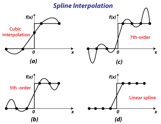
A piecewise polynomial (parametric) curvature is more commonly referred to as a spline in the computer engineering subdisciplines of computer-aided modeling and computer graphics. Splines are commonly used in various domains due to their ease of creation, ease and accuracy of evaluation, and ability to estimate complicated shapes via curve fitting and highly interactive curve design.
Splines are bendable spline tools used by shipping companies and draughtsmen to construct smooth shapes. A spline is a particular function defined piecewise using polynomials in mathematics. Spline interpolation is frequently clearly favored to polynomial interpolation in many situations because it produces similar outcomes even when employing lower degree polynomials while preventing Runge's phenomena for higher degrees.
A piecewise trendline is what a Spline is. Trying to fit a single regression line to a set of data that is particularly dynamic can lead to a lot of tradeoff. You can modify your trend line to fit nicely in one place, but you may end up overfitting in plenty of other regions as a result. Instead, we divide the data into "knots" and fit a new regression line to each segment divided by the knots or division points.
A spline model of the curve is generated first, and afterwards the spline is produced at the desired locations in spline interpolation. The spline interpretation of a curve in a 2-dimensional surface is found using the function splrep.
Methods For Spline 1-D Interpolation
| BSpline(t, c, k[, extrapolate, axis]) | B-spline basis with a univariate spline. |
| make_interp_spline(x, y[, k, t, bc_type, …]) | Calculate the interpolating B-spline (coefficients). |
| make_lsq_spline(x, y, t[, k, w, axis, …]) | Calculate an LSQ B |
Functional interface:
| splrep(x, y[, w, xb, xe, k, task, s, t, …]) | Find a 1-D curve's B-spline representation. |
| splprep(x[, w, u, ub, ue, k, task, s, t, …]) | Find the N-D curve's B-spline representation. |
| splev(x, tck[, der, ext]) | Determine the value of a B-spline or its derivatives. |
| splint(a, b, tck[, full_output]) | Calculate a B-definite spline's integral between two points. |
| sproot(tck[, mest]) | Find the cubic B-roots. spline's |
| spalde(x, tck) | Evaluate all of a B-derivatives. spline's |
| splder(tck[, n]) | Calculate the spline form of a spline's derivative. |
| splantider(tck[, n]) | Calculate the spline for a given spline's antiderivative (integral). |
| insert(x, tck[, m, per]) | In a B-spline, tie knots. |
Object-oriented FITPACK interface:
| UnivariateSpline(x, y[, w, bbox, k, s, ext, …]) | Fitting a 1-D smoothing curve to a large number of observations. |
| InterpolatedUnivariateSpline(x, y[, w, …]) | For a given collection of data points, a 1-D interpolating spline is used. |
| LSQUnivariateSpline(x, y, t[, w, bbox, k, …]) | Internal knots in a one-dimensional spline. |
2-D Splines
If data is available on a grid
| RectBivariateSpline(x, y, z[, bbox, kx, ky, s]) | Over a rectangular grid, a bivariate spline approximation is used. |
| RectSphereBivariateSpline(u, v, r[, s, …]) | On a rectangular grid on a sphere, this function applies a bivariate spline approximation is used. |
If available data is unstructured.
| BivariateSpline() | Bivariate splines' base class. |
| SmoothBivariateSpline(x, y, z[, w, bbox, …]) | Approximation with a smooth bivariate spline. |
| SmoothSphereBivariateSpline(theta, phi, r[, …]) | In spherical coordinates, a smooth bivariate spline approximation. |
| LSQBivariateSpline(x, y, z, tx, ty[, w, …]) | Bivariate spline approximation using weighted least-squares. |
| LSQSphereBivariateSpline(theta, phi, r, tt, tp) | In spherical coordinates, Bivariate spline approximation using weighted least-squares. |
| bisplev(x, y, tck[, dx, dy]) | Calculate the derivatives of a bivariate B-spline. |
Interpolation using Radial Base Function
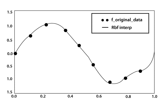
Many fields employ interpolation and approximation techniques. Basic interpolation and approximate solution methods rely on "having ordered," which refers to tessellation in n-dimensional data in general, such as sorting, triangulation, and the creation of tetrahedral meshes, among other things. In the case of d-dimensional tessellation, the algorithms are quite complicated. Meshfree (gridless) approaches using Radial Basis Functions, on the other hand, can be used to perform interpolation and approximation (RBF). In general, the RBF interpolation approaches result in a linear system of equations solution.
RBF interpolation is an effective approach in approximation theory for creating higher-degree precise interpolants of unstructured data in potentially high-dimensional environments. The interpolant is a weighted sum of a radial basis function, such as those seen in Gaussian distributions. RBF interpolation is a grid-free approach, which means that the terminals (points in the domain) do not have to be on a structured grid and no mesh construction is required. Even in high dimensions, it is frequently spectrally precise and stable for huge numbers of nodes.
RBF interpolation is one of many interpolation approaches that can be utilised as the theoretical underpinning of methods for approximating linear operators. Differential operators, and surface differential operators and integral operators have all been approximated using RBF interpolation.
In contrast to inverse distance weighting (IDW), RBFs produce smoother and less oscillatory interpolation. Colour calibration, Animation blending, Surface reconstruction, facial retargeting, and other applications in Computer Graphics. Despite the diversity of its uses, scattered data interpolation is a common thread that runs through them all.