Prior and Posterior Gaussian Process for Different Kernels in Scikit Learn

What is the Gaussian Process?

A Gaussian process, which is used in probability theory and statistics, is a stochastic procedure (a group of random variables listed by time or space) in which every finite collection of those random variables has a multivariate normal distribution, or in other words, every finite linear combination of them has a normal distribution. A Gaussian process's distribution is the sum of all of those (infinitely many) random variables, and it is a distribution over functions having a continuous domain, such as time or space. Gaussian processes can be viewed as an infinite-dimensional generalization of multivariate normal distributions.

Statistical models can profit from the features of Gaussian processes inherited from the normal distribution. For instance, if a random process is treated as a Gaussian process, it is possible to get the distributions of various derived values explicitly. These figures consist of the process's average value over several iterations and the error introduced by predicting the average from a limited sample of iterations' sample values. As the amount of data rises, accurate models frequently scale poorly, but numerous approximation techniques have been established that frequently maintain acceptable accuracy while significantly lowering computing time.

What are the Prior and Posterior Gaussian processes?

Predictions regarding the function that produced the data are made using the Gaussian process regression method and the idea of a prior and posterior distribution. The original opinion in the function is represented by the prior distribution and is held prior to any data being recorded, whereas the revised belief is represented by the posterior distribution and is held following the observation of any data.

The Gaussian process kernel and mean functions are collectively referred to as the prior distribution's defining characteristics. The user can define these parameters or let the data estimate them. The posterior distribution is then determined using Bayesian inference based on the observed data and the prior distribution.

The function's modified conviction can be predicted at new input points using the posterior distribution, which represents the updated belief based on the observed data. The forecasts are derived through sampling from the posterior distribution, which provides a range of potential functions that might have produced the observed data. It is possible to anticipate the output value using the mean of these functions and to determine the degree of uncertainty in the predictions; one can calculate the variance of the functions.

Different Kernels in Scikit Learn

The GaussianProcessRegressor class in Scikit-Learn may be employed to implement Gaussian process regression. This class gives you the option to select the kind of covariance function (often referred to as a kernel) you would like to employ. The squared exponential kernel (commonly known as the Radial Basis Function, or RBF) kernel, the Matern kernel, and the periodic kernelare a few popular kernels that are offered in Scikit-Learn.

Squared Exponential Kernel

The squared exponential kernel also called the Radial Basis Function (RBF) kernel, is a preferred option for many regression issues. It is a smooth, stationary kernel that is defined as follows:

k * (x_{1}, x_{2}) = e ^ (- 1/2 * ((x_{1} - x_{2})/l))

where x1 and x2 are input points, and l is the kernel's length scale.

As it is smooth and has a constant length scale, the squared exponential kernel is a good choice for modeling functions that change gradually. It is also a stationary kernel, which means that it is not dependent on the absolute values of the input points but instead on the distances between them.

Example code for the Squared Exponential Kernel

imports pandas as pd

from sklearn.model_selection import train_test_split

from sklearn.metrics import roc_auc_score as ras

data = pd.read_csv(

    "https://raw.githubusercontent.com/lucifertrj/"

    "100DaysOfML/main/Day14%3A%20Logistic_Regression"

    "_Metric_and_practice/heart_disease.csv")

X = data.drop("target", axis=1)

y = data['target']

X_train, X_test,\

y_train, y_test = train_test_split(X, y, test_size=0.25, random_state=42)

In scikit-learn, the squared exponential kernel may be applied to the GaussianProcessRegressor class using the RBF kernel class, as illustrated in the example below:

from sklearn.gaussian_process import GaussianProcessRegressor

from sklearn.gaussian_process.kernels import RBF

# Creating the squared exponential (RBF) kernel

kernel = RBF()

# Creating the Gaussian process regressor with the RBF kernel

gpr = GaussianProcessRegressor(kernel=kernel)

# Fitting the model to the data

gpr.fit(X_train, y_train)

# Making predictions on the test set

y_pred = gpr.predict(X_test)

ras(y_test, y_pred)

Output

0.7055226480836237

Remember that you might need to adjust the kernel's length scale to get the best results for your particular data and prediction task.

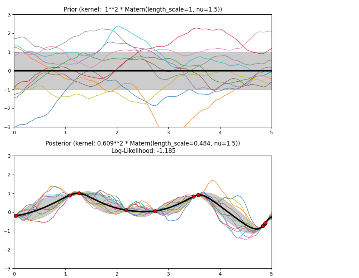
Matern Kernel

The Matern kernel is a generalization of the squared exponential kernel that can be applied to issues where the data might not be smooth. It is described as follows:

k(r,l)=( (1+ sqrt(3)⋅r)/l )e^(- ( sqrt(3)⋅r)/ l )

Here l is the length scale of the kernel, x1 and x2 are the input points, and r is the Euclidean distance between them.

r = √(x1- x2)²+(y1-y2)²

The smoothness of the Matern kernel is controlled by the two parameters nu and l. The parameter nu determines the differentiability of the kernel; differentiable kernels are those with more significant values of nu. The length scale of the kernel, or parameter l, determines how rapidly the kernel decays to zero as the separation between the input points widens.

By utilizing the Matern kernel class in scikit-learn, the Matern kernel may be utilized with the GaussianProcessRegressor class, as demonstrated in the example below:

Example code for Matern Kernel

imports pandas as pd

from sklearn.model_selection import train_test_split

from sklearn.metrics import roc_auc_score as ras

data = pd.read_csv(

    "https://raw.githubusercontent.com/lucifertrj/"

    "100DaysOfML/main/Day14%3A%20Logistic_Regression"

    "_Metric_and_practice/heart_disease.csv")

X = data.drop("target", axis=1)

y = data['target']

X_train, X_test,\

y_train, y_test = train_test_split(X, y, test_size=0.25, random_state=42)

from sklearn.gaussian_process import GaussianProcessRegressor

from sklearn.gaussian_process.kernels import Matern

# create the Matern kernel

kernel = Matern()

# create the Gaussian process regressor with the Matern kernel

gp = GaussianProcessRegressor(kernel=kernel)

# fit the model to the data

gp.fit(X_train, y_train)

# make predictions on the test set

y_pred = gp.predict(X_test)

ras(y_test, y_pred)

Output

0.7226480836236934

Remember that the Matern kernel's parameters (nu and l) may need to be adjusted to get the most remarkable performance on your particular data and prediction task.

Periodic Kernel or ExpSineSquared

A kernel that is helpful for simulating periodic functions is the periodic kernel. It is defined as follows:

k(x_{1}, x_{2}) = e ^ (- 2sin^2 (pi * |x_{1} - x_{2}|/p))

where x1 and x2 are input points, and p denotes the kernel's period.

The periodic kernel contains a single parameter, p, which determines how long the kernel will run. This parameter determines the kernel's ability to simulate the periodic function's cycle length.

Using the Periodic kernel class in scikit-learn, the periodic kernel may be applied to the GaussianProcessRegressor class, as demonstrated in the example below:

Example Code for Periodic Kernel or ExpSineSquared

from sklearn.datasets import make_friedman2

from sklearn.gaussian_process import GaussianProcessRegressor

from sklearn.gaussian_process.kernels import ExpSineSquared

X, y = make_friedman2(n_samples=50, noise=0, random_state=0)

kernel = ExpSineSquared(length_scale=1, periodicity=1)

gpr = GaussianProcessRegressor(kernel=kernel, alpha=5,

random_state=0).fit(X, y)

gpr.score(X, y)

Output

0.014494116027408799

To get the best results on your particular data and prediction task, note that the periodic kernel's period (p) may need to be adjusted.

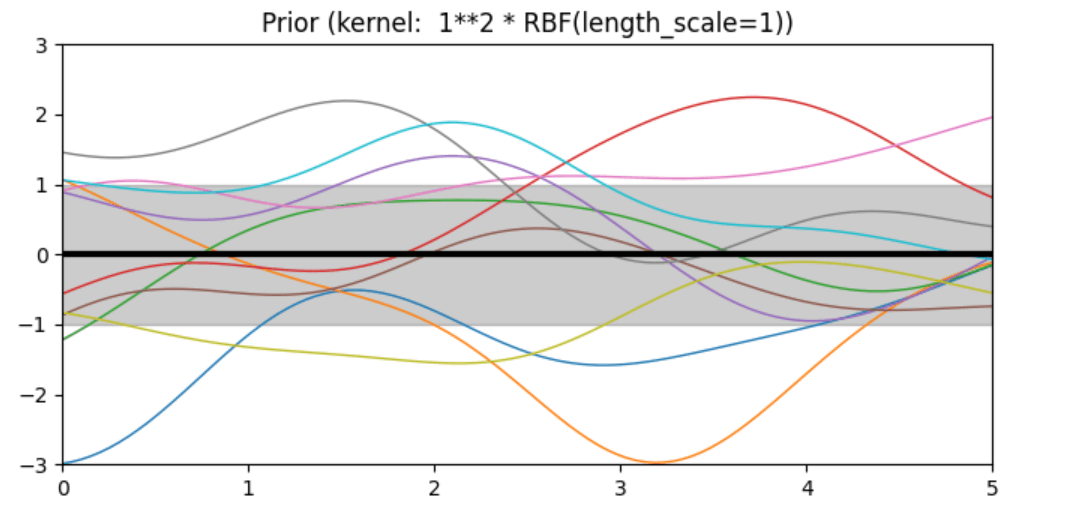
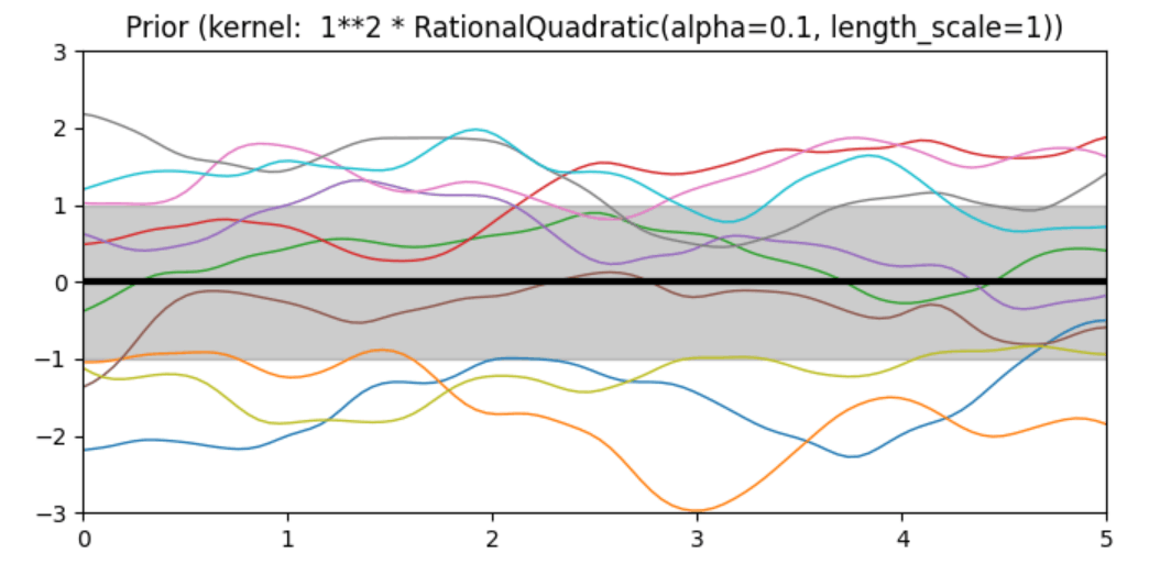
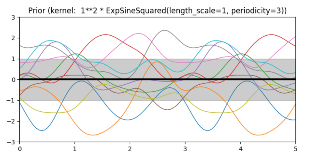
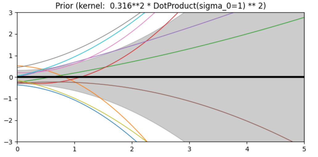
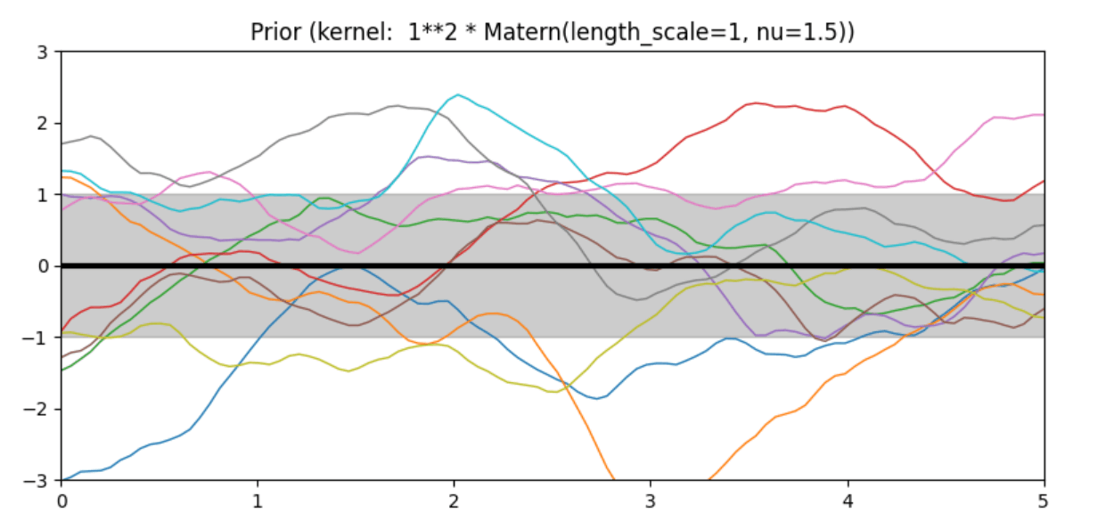
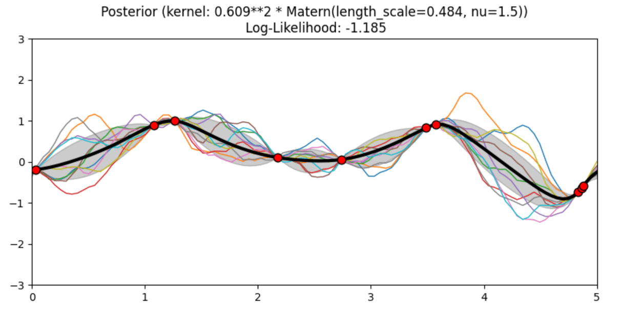
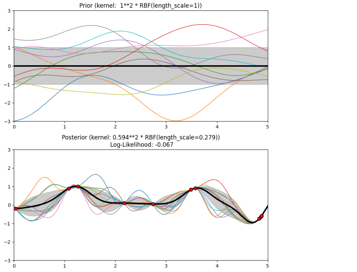
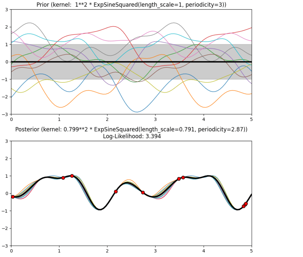
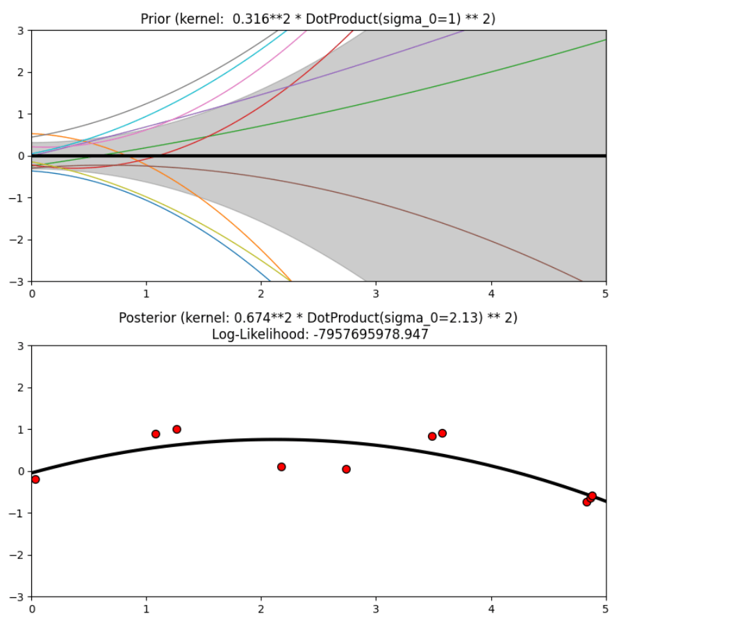
Description of prior and posterior Gaussian process for different kernels

The prior and posterior of a GPR with various kernels are demonstrated in this example. For both prior and posterior, standard deviation, mean, and 10 samples are depicted.

In this example, along with the above-discussed three kernels, we also have the prior and posterior of a GPR with some other kernels like the Rational Quadratic Kernel and the DotProduct Kernel.

Code

import numpy as np

from matplotlib import pyplot as plt

from sklearn.gaussian_process import GaussianProcessRegressor

from sklearn.gaussian_process.kernels import (RBF, Matern, RationalQuadratic,

ExpSineSquared, DotProduct, ConstantKernel)

kernels = [1 * RBF(length_scale=1.0, length_scale_bounds=(1e-1, 10.0)),

           1 * RationalQuadratic(length_scale=1.0, alpha=0.1),

           1 * ExpSineSquared(length_scale=1.0, periodicity=3.0,

                                length_scale_bounds=(0.1, 10.0),

                                periodicity_bounds=(1.0, 10.0)),

           ConstantKernel(0.1, (0.01, 10.0))

               * (DotProduct(sigma_0=1.0, sigma_0_bounds=(0.1, 10.0)) ** 2),

           1 * Matern(length_scale=1.0, length_scale_bounds=(1e-1, 10.0),

                        nu=1.5)]

for kernel in kernels:

gpr = GaussianProcessRegressor(kernel=kernel)

    plt.figure(figsize=(8, 8))

    plt.subplot(2, 1, 1)

    X_ = np.linspace(0, 5, 100)

    y_m, y_std = gpr.predict(X_[:, np.newaxis], return_std=True)

    plt.plot(X_, y_m, 'k', lw=3, zorder=9)

    plt.fill_between(X_, y_m - y_std, y_m + y_std,

                     alpha=0.2, color='black')

    y_s = gpr.sample_y(X_[:, np.newaxis], 10)

    plt.plot(X_, y_s, lw=1)

    plt.xlim(0, 5)

    plt.ylim(-3, 3)

    plt.title("Prior (kernel:  %s)" % kernel, fontsize=12)

rg = np.random.RandomState(4)

    X = rg.uniform(0, 5, 10)[:, np.newaxis]

    y = np.sin((X[:, 0] - 2.5) ** 2)

    gpr.fit(X, y)

    plt.subplot(2, 1, 2)

    X_ = np.linspace(0, 5, 100)

    y_m, y_std = gpr.predict(X_[:, np.newaxis], return_std=True)

    plt.plot(X_, y_m, 'k', lw=3, zorder=9)

    plt.fill_between(X_, y_m - y_std, y_m + y_std,

                     alpha=0.2, color='k')

    y_s = gpr.sample_y(X_[:, np.newaxis], 10)

    plt.plot(X_, y_s, lw=1)

    plt.scatter(X[:, 0], y, c='red', s=60, zorder=20, edgecolors=(0, 0, 0))

    plt.xlim(0, 5)

    plt.ylim(-3, 3)

    plt.title("Posterior (kernel: %s)\n Log-Likelihood: %.3f"

              % (gpr.kernel_, gpr.log_marginal_likelihood(gpr.kernel_.theta)),

              fontsize=12)

    plt.tight_layout()

plt.show()

Output

Conclusion

In conclusion, choosing the appropriate kernel for your data and prediction goal can help your model be more accurate. Gaussian process regression and the choice of the kernel are crucial tools for modeling functions in Scikit-Learn.