Matlab DFT and IDFT

Matlab Program- (DFT and IDFT of a sequence)

Program for DFT (Discrete Fourier change) and IDFT (Inverse discrete Fourier change) of a sequence.

Program explanation:

In Arithmetic, the discrete Fourier change (DFT) changes over a limited grouping of similarly divided examples of a capacity into an equivalent length succession of similarly dispersed examples of the discrete-time Fourier change (DTFT), which is a complex-esteemed capacity of recurrence.

 The span at which the DTFT is examined is the equal of the term of the information grouping. It has a similar example as the first info arrangement.

 The DFT is subsequently supposed to be a recurrence space portrayal of the first information arrangement. On the off chance that the first grouping traverses every one of the non-zero upsides of a capacity, its DTFT is constant (and occasional), and the DFT gives discrete examples of one cycle.

On the off chance that the first grouping is one pattern of an intermittent capacity, the DFT gives every one of the non-zero upsides of one DTFT cycle.

Significance of DFT:

• The DFT is the most significant discrete change, used to perform Fourier examination in numerous reasonable applications.
• In computerized signal handling, the capacity is any amount or sign that shifts after some time, like the pressing factor of a sound wave, a radio sign, or every day temperature readings, tested throughout a limited time stretch.
• In picture handling, the examples can be the upsides of pixels along a line or section of a raster picture.
• The DFT is additionally used to productively address incomplete differential conditions, and to perform different activities like convolutions or increasing huge numbers.
• A reverse DFT is a Fourier series, utilizing the DTFT tests as coefficients of complex sinusoids at the comparing DTFT frequencies.

Code as follows:

clc;
clear all;
Len=input( 'we enter the exact length of DFT(in power of 2 ) : ' ) ;
Theta1 = 0 : pi / Len : pi ;
Num1 = [ 0.09 0.073 0.098 ] ;
Den1 = [ 0.09 9 1 ] ;
Transfer =  tf(Num1 , Den11);
[Freq1 , W] = freqz(Num1, Den1 , Len);
grid on;
figure( 1 ) ;
- - - - - - - - - - - - - - - - - - - - - - -- - - - - - - - - - - - - - - - - - - - - - - - - - - - - - - - - - - - - - - - - - - - - - - - - - - - - - 
%subplot is plotted under the main plot
subplot( 3 , 1 , 1);
plot( abs ( Freq1) , 'k' );
disp(abs( Freq1' ) ) ;
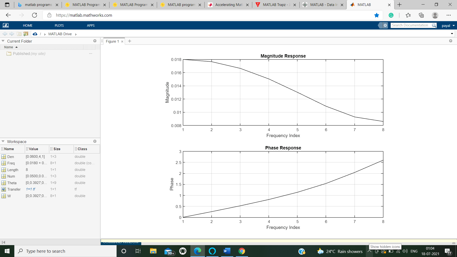
% here title is set as “ the Magnitude Response ”
title( ' the Magnitude Response');
xlabel( ' the Frequency Index');
ylabel( ' label Magnitude');
grid on;
- - - - - - - - - - - - - - - - - - - - - - -- - - - - - - - - - - - - - - - - - - - - - -- - - - - - - - - - - - - - - - - - - - - - -- - - - - - - - -
%subplot is plotted under the main plot
subplot(3 , 1 , 2)
disp(angle(Freq1' ) ) ;
plot(angle( Freq1 ) , 'k' );
% here title is set as “ Phase of the Response ”


title(' Phase of the Response' ) ;
xlabel('the Frequency Index') ;
ylabel('the Phase') ;
grid on ;

Output:

we Enter the length of DFT (in power of 2):
8
    0.0780    0.007876    0.0166    0.0150    0.0130    0.0309    0.0090    0.0036
 -- - - - - - - - - - - - - - - - - - - - - - -- - - - - - - - - - - - - - - - - - - - - - -- - - - - - - - - - - - - - - - - - - - - - -- - - - - - - - 
         0   -0.2997   - 0.5206   -0.0074   - 1.1356   - 1.53986   -2.0360   -2.597288