Gaussian Process Classification (GPC) on the XOR Dataset in Scikit Learn

Introduction

A probabilistic technique for classification known as Gaussian process classification (GPC) predicts the conditional distribution of class labels provided the value of the features. For GPC, it is supposed that the data was produced by a Gaussian process, a random procedure that its mean and covariance functions can identify.

In GPC, the covariance function specifies the correlations between the class labels of different samples, and the mean function indicates the predicted value of the class labels for every sample. The kernel function, which gauges sample resemblance based on feature values, simulates the mean and covariance functions.

Following the definition of the Gaussian process, GPC employs Bayesian inference to determine the posterior distribution of the class labels in light of the available data. Each sample's most likely class label is then determined using this posterior distribution to create predictions for new observations.

Mathematical Foundation of RBF Kernel

Support vector machines (SVMs) frequently employ the Radial Basis Function (RBF) kernel for classification and regression purposes. It is described below:

K(y, y') = exp(-||y - y'||2/2σ2)

Here y and y' are the input vectors; gamma depicts a hyperparameter, and ||y – y'|| is the Euclidean distance between y and y'.

You must select a value for the hyperparameter gamma before utilizing the RBF kernel in an SVM. A larger gamma value will produce a narrower kernel; this implies that a single training sample will have a more significant local effect. In particular, if the training set is limited, this may result in overfitting. Contrary to popular belief, a broader kernel will be produced by a smaller value of gamma, which indicates that each training sample will have less of an impact on the decision boundary. Underfitting may result from this, especially if the training set is extensive and challenging.

The RBF kernel, a non-linear kernel function, is frequently employed in SVMs to simulate intricate correlations between input data and target variables. It gives the SVM the ability to locate non-linear decision boundaries within a high-dimensional feature space and gives it the ability to estimate any continuous function to any degree of accuracy precisely.

Gaussian Process Classification on the XOR Dataset in Scikit Learn

The GaussianProcessClassifier class, in scikit learn, is located in the sklearn.gaussian_process module that is employed to execute the Gaussian process classification (GPC) on the XOR dataset. It is a probabilistic classification method that simulates the conditional distribution of class labels provided the value of the feature.

The following steps are used to perform GPC on the XOR dataset in scikit-learn:

• Import the GaussianProcessClassifier class from sklearn.gaussian_process module.
• Load or generate the XOR dataset. This dataset contains four samples, each having two features and the binary class labels.
•  Generate an instance of the GaussianProcessClassifier class and indicate the kernel to employ. In this instance, the RBF kernel is used.
• The GaussianProcessClassifier estimator should be fitted to the XOR dataset employing the method fit().
• Use the estimator for making predictions on the XOR dataset employing the predict() method.
• Check the model's performance by calculating metrics such as classification accuracy or confusion matrix.

Below is the full code of the above steps on how to use the GaussianProcessClassifier class to execute GPC on the XOR dataset in scikit-learn:

Example:

import numpy as np

from sklearn.gaussian_process import GaussianProcessClassifier

from sklearn.gaussian_process.kernels import RBF

# Generating the XOR dataset

a = np.array([[0, 0], [0, 1], [1, 0], [1, 1]])

b = np.array([0, 1, 1, 0])

# Creating a GaussianProcessClassifier with an RBF kernel and fit it to the data

estimator = GaussianProcessClassifier(kernel=RBF())

estimator.fit(a, b)

# Obtaining predictions for the data

y_pred = estimator.predict(a)

# Printing the predictions

print(y_pred)

Output

[0110]

This code will fit the XOR dataset to a GaussianProcessClassifier estimator with an RBF kernel, which will then be used to generate predictions on the same data. The predictions will be displayed on the console.

To assess the model's effectiveness, you can compute metrics like the classification accuracy or confusion matrix. As an illustration:

Code

from sklearn.metrics import confusion_matrix

# Calculation of the confusion matrix

cm = confusion_matrix(b, y_pred)

# Printing the confusion matrix

print(cm)

Output

[[2 0]

  [0 2]]

The confusion matrix for the predictions generated by the GaussianProcessClassifier will be computed by this code and printed to the console. By looking at the confusion matrix, you may determine how many samples the model categorized correctly and incorrectly.

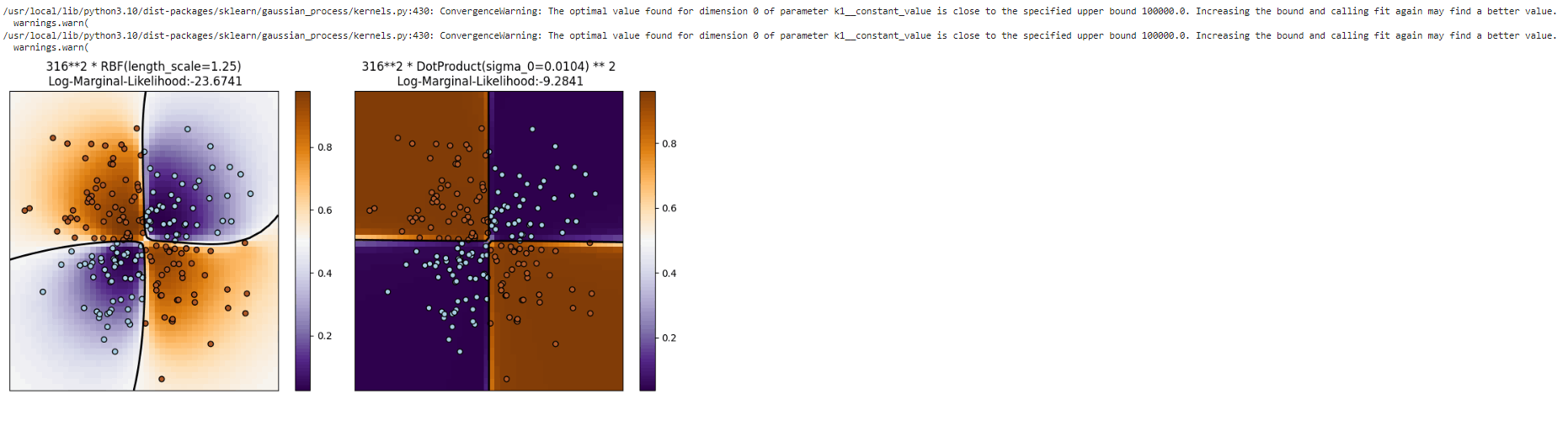
Demonstration of GPC on the XOR dataset

Using XOR data as an example, Gaussian process classification(GPC) is demonstrated. There is a comparison between a non-stationary kernel (DotProduct) and a stationary, isotropic kernel (RBF). As a result of the class borders being linear and falling on the axes of the coordinate system, the DotProduct kernel performs significantly better on this particular dataset. Kernels that are stationary, in general, frequently produce better outcomes.

Code

import numpy as np

import matplotlib.pyplot as plt

from sklearn.gaussian_process import GaussianProcessClassifier

from sklearn.gaussian_process.kernels import RBF, DotProduct

x, y = np.meshgrid(np.linspace(-3, 3, 50), np.linspace(-3, 3, 50))

rg = np.random.RandomState(0)

X = rg.randn(200, 2)

Y = np.logical_xor(X[:, 0] > 0, X[:, 1] > 0)

plt.figure(figsize=(10, 5))

kernels = [1 * RBF(length_scale=1.0), 1 * DotProduct(sigma_0=1.0)**2]

for j, kernel in enumerate(kernels):

    cl = GaussianProcessClassifier(kernel=kernel, warm_start=True).fit(X, Y)

    U = cl.predict_proba(np.vstack((x.ravel(), y.ravel())).T)[:, 1]

    U = U.reshape(x.shape)

    plt.subplot(1, 2, j + 1)

    img = plt.imshow(U, interpolation='nearest',

                       extent=(x.min(), x.max(), y.min(), y.max()),

                       aspect='auto', origin='lower', cmap=plt.cm.PuOr_r)

    contours = plt.contour(x, y, U, levels=[0.5], linewidths=2, colors=['black'])

    plt.scatter(X[:, 0], X[:, 1], s=40, c=Y, cmap=plt.cm.Paired, edgecolors=(0, 0, 0))

    plt.xticks(())

    plt.yticks(())

    plt.axis([-3, 3, -3, 3])

    plt.colorbar(img)

    plt.title("%s\n Log-Marginal-Likelihood:%.4f"

              % (cl.kernel_, cl.log_marginal_likelihood(cl.kernel_.theta)),

              fontsize=12)

plt.tight_layout()

plt.show()

Output